Filling in Python's gaps in statistics packages with Rmagic
Published on January 15, 2013 by Dr. Randal S. Olson
ipython pandas python R language Rmagic statistics tutorial
5 min READ
Have you ever found yourself searching for a statistics package in Python, but it just isn't available? This is the biggest reason I've heard when my colleagues say they're unwilling to make the switch from R to Python for statistical analysis. To counteract that argument, the geniuses developing IPython created Rmagic, a package which allows you to run R code within the IPython interface.
Let's get to the cut and dry and see how it works. If you want to follow along, the IPython Notebook and data file is available on github: https://github.com/rhiever/rmagic-tutorial
Installing Rmagic
Rmagic comes along with the IPython package, so just follow my IPython tutorial to install IPython. Beyond IPython, all you need is Python's rpy2 package to run Rmagic:
sudo easy_install rpy2
I also exclusively use the pandas package when I'm dealing with data, so make sure to have that installed as well:
sudo easy_install pandas
Using Rmagic for statistical analysis
I do most of my statistical analysis in Python nowadays, but sometimes there's just that one statistical function that I need that Python doesn't quite have yet. In those cases, I use Rmagic to "fill the gap" in Python's statistics packages. Rmagic lets me pass my data to R, run the R function on the data, then seamlessly return the data back to Python before I start having nightmares about using R again. Since there are already a ton of R statistics tutorials out there, this tutorial will instead concentrate on how to use Rmagic to link together Python and R code.
Load the rmagic extension
%load_ext rmagic
Use R to view summary information about the data
If you like how R provides summary information about the data, you can print out the summary() function.
%R tells IPython that the line is R code.
-i parasiteData tells IPython to pass the parasiteData DataFrame to R.
The rest is R code. You can have multiple lines of R code separated by semicolons.
Note that when you want to print anything out from R, you need to place the print() function around it.
from pandas import *

# read data from data file into a pandas DataFrame
parasiteData = read_csv("parasite_data.csv", sep=",", na_values=["", " "])

# print the R summary() function for the data
%R -i parasiteData print(summary(parasiteData))


   Virulence      Replicate    ShannonDiversity
 Min.   :0.50   Min.   : 1.0   Min.   :0.0000
 1st Qu.:0.60   1st Qu.:13.0   1st Qu.:0.0000
 Median :0.75   Median :25.5   Median :0.8457
 Mean   :0.75   Mean   :25.5   Mean   :0.8364
 3rd Qu.:0.90   3rd Qu.:38.0   3rd Qu.:1.5337
 Max.   :1.00   Max.   :50.0   Max.   :2.9008
 NA's   :50
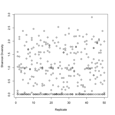
View a R plot in IPython
You can even view plots of your data in IPython from R.
from pandas import *

# read data from data file into a pandas DataFrame
parasiteData = read_csv("parasite_data.csv", sep=",", na_values=["", " "])

# plot the Shannon Diversity as a function of Virulence in R
%R -i parasiteData plot(ShannonDiversity ~ Replicate, data = parasiteData,
                        xlab="Replicate",
                        ylab="Shannon Diversity")

Filling in the gaps
Beyond the basics, you can use R to perform a single function on your data, then return the result back to Python. Here's a simple example.
-o meanShannonDiversity tells IPython to return the meanShannonDiversity variable back from R to IPython.
from pandas import *

# read data from data file into a pandas DataFrame
parasiteData = read_csv("parasite_data.csv", sep=",", na_values=["", " "])

# calculate the mean Shannon Diversity for experiments with Virulence = 0.7
# do the subsetting in Python - it's easier!
ShannonDiversity = parasiteData[parasiteData["Virulence"] == 0.7]["ShannonDiversity"]

%R -i ShannonDiversity -o meanShannonDiversity meanShannonDiversity <- mean(ShannonDiversity)

print "R Mean:     ", meanShannonDiversity[0]
print "Python Mean:", ShannonDiversity.mean()


R Mean:      1.1261538832
Python Mean: 1.1261538832
How about a more useful example? We can use R's built-in bootstrapping function to construct 95% confidence intervals for our data.
from pandas import *

# read data from data file into a pandas DataFrame
parasiteData = read_csv("parasite_data.csv", sep=",", na_values=["", " "])

# calculate the 95% confidence interval for Shannon Diversity for
# experiments with Virulence = 0.5 and 0.8
# do the subsetting in Python - it's easier!
ShannonDiversityV5 = parasiteData[parasiteData["Virulence"] == 0.5]["ShannonDiversity"]
ShannonDiversityV8 = parasiteData[parasiteData["Virulence"] == 0.8]["ShannonDiversity"]

# load R's boot library
%R require(boot)

# define the function we're bootstrapping (mean)
%R sampleMean <- function(x, d) { return(mean(x[d])) }

# bootstrap the 95% confidence intervals for the Virulence = 0.5 experiments
%R -i ShannonDiversityV5 -o bootstrapCIV5
%R bootstrap <- boot(ShannonDiversityV5, sampleMean, R=10000);
%R ci <- boot.ci(bootstrap, type="basic");
$R bootstrapCIV5 <- list(ci$basic[1,4], ci$basic[1,5])

# bootstrap the 95% confidence intervals for the Virulence = 0.8 experiments
%R -i ShannonDiversityV8 -o bootstrapCIV8
%R bootstrap <- boot(ShannonDiversityV8, sampleMean, R=10000);
%R ci <- boot.ci(bootstrap, type="basic");
%R bootstrapCIV8 <- list(ci$basic[1,4], ci$basic[1,5])

# plot the 95% confidence intervals
figure(figsize(8,6))
xlim(0.4, 0.9)
title("Comparison of Shannon Diversity")
xlabel("Virulence")
ylabel("Shannon Diversity")
errorbar(x = [0.5], y = [ShannonDiversityV5.mean()],
         yerr = [ShannonDiversityV5.mean() - bootstrapCIV5[0],
                 bootstrapCIV5[1] - ShannonDiversityV5.mean()])
errorbar(x = [0.8], y = [ShannonDiversityV8.mean()],
         yerr = [ShannonDiversityV8.mean() - bootstrapCIV8[0],
                 bootstrapCIV8[1] - ShannonDiversityV8.mean()])

# print the 95% confidence intervals
print "95% confidence interval (Virulence = 0.5):",
       bootstrapCIV5[0], "to", bootstrapCIV5[1]
print "95% confidence interval (Virulence = 0.8):",
       bootstrapCIV8[0], "to", bootstrapCIV8[1]


Loading required package: boot
95% confidence interval (Virulence = 0.5): [ 0.55618822] to [ 0.92704398]
95% confidence interval (Virulence = 0.8): [ 1.05437854] to [ 1.49182085]

And there you have it: we know there is a significant difference between the experiments with Virulence = 0.5 and 0.8 because their 95% confidence intervals don't overlap.
For those who use Octave, there is a similar octavemagic package in IPython as well.