Using pandas DataFrames to process data from multiple replicate runs in Python


Published on June 26, 2012 by Dr. Randal S. Olson

data management pandas plotting data python research statistics

5 min READ


Per a recommendation in my previous blog post, I decided to follow up and write a short how-to on how to use pandas to process data from multiple replicate runs in Python.

If you do research like mine, you'll often find yourself with multiple datasets from an experiment that you've run in replicate multiple times. There are plenty of ways to manage and process data nowadays, but I've never seen it made so easy as it is with pandas.

Installing pandas

If you don't already have pandas installed, download it at: https://pandas.pydata.org/getting_started.html

Then do the typical python package install process.

cd unzipped-pandas-folder-name/
python setup.py build_ext --inplace
sudo python setup.py install

Note: if you're not using pandas in IPython Notebook, the build_ext --inplace part is unnecessary.

Using pandas

Below, I'll show you the 23 lines of Python code that I use to read in, process, and plot all of the data from my experiments. After that, I'll break the code block down line-by-line and explain what's happening.

from pandas import *
import glob

dataLists = {}

# read data
for folder in glob.glob("experiment-data-directory/*"):
    
    dataLists[folder.split("/")[1]] = []
    
    for datafile in glob.glob(folder + "/*.csv"):

        dataLists[folder.split("/")[1]].append(read_csv(datafile))

# calculate stats for data
meanDFs = {}
stderrDFs = {}

for key in dataLists.keys():
    
    keyDF = (concat(dataLists[key], axis=1, keys=range(len(dataLists[key])))
            .swaplevel(0, 1, axis=1)
            .sortlevel(axis=1)
            .groupby(level=0, axis=1))
    
    meanDFs[key] = keyDF.mean()
    stderrDFs[key] = keyDF.std().div(sqrt(len(dataLists[key]))).mul(2.0)
    
    keyDF = None

# plot data
for column in meanDFs[key].columns:
    
    # don't plot generation over generation - that's pointless!
    if not (column == "generation"):
    
        figure(figsize=(20, 15))
        title(column.replace("_", " ").title())
        ylabel(column.replace("_", " ").title())
        xlabel("Generation")
        
        for key in meanDFs.keys():

            errorbar(x=meanDFs[key]["generation"], y=meanDFs[key][column], yerr=stderrDFs[key][column], label=key)
            
        legend(loc=2)

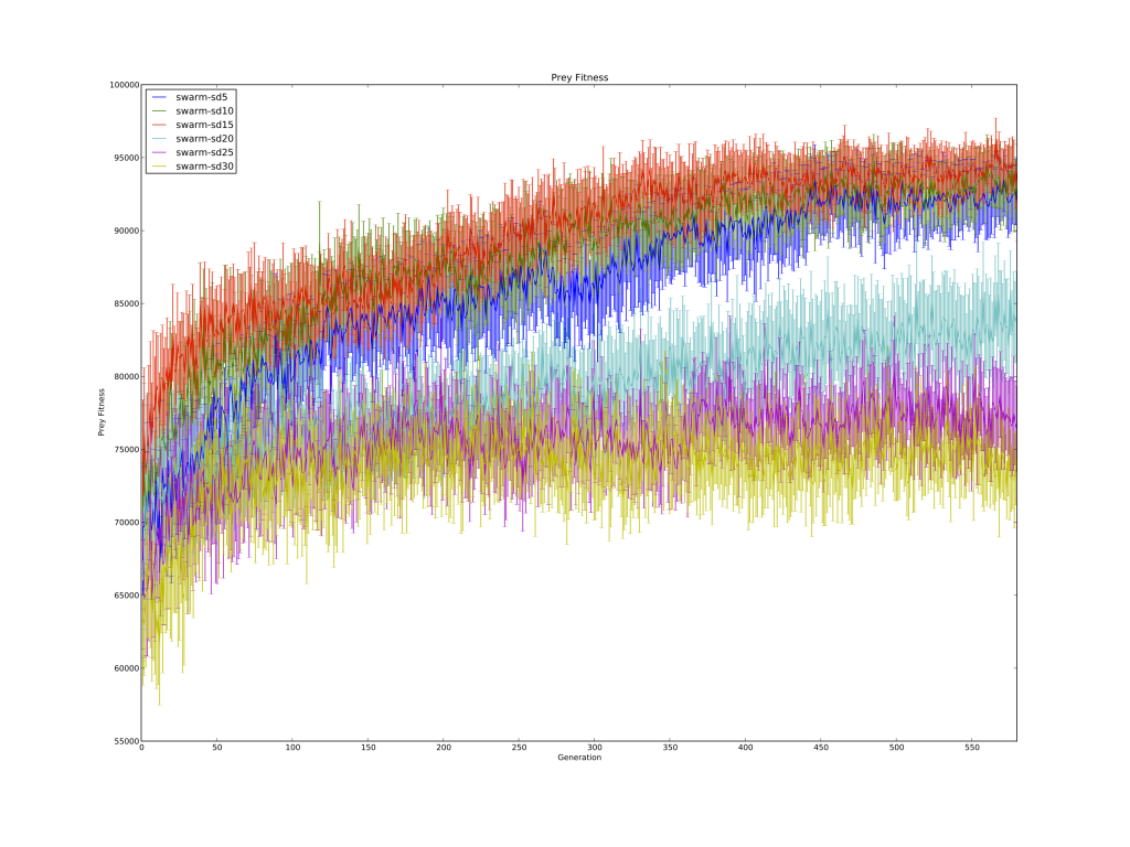
Here's one graph from the end product.

Prey Fitness

Required packages

Along with the pandas package, the glob package is extremely useful for aggregating folders and files into a single list so they can be iterated over.

from pandas import *
import glob

Reading data with pandas

glob.glob(str) aggregates all of the files and folders matching a given *nix directory expression.

for folder in glob.glob("experiment-data-directory/*"):

For example, say experiment-data-directory contains 4 other directories: treatment1, treatment2, treatment3, and treatment 4. It will return a list of the directories in string format.

print glob.glob("experiment-data-directory/*")
>>> ["treatment1", "treatment2", "treatment3", "treatment 4"]

Similarly, glob.glob(folder + "/*.csv") will return a list of all .csv files in the given directory.

print glob.glob("treatment1/*.csv")
>>> ["treatment1/run1.csv", "treatment1/run2.csv", "treatment1/run3.csv"]

Finally, line 13 stores all of the pandas DataFrames read in by the pandas read_csv(str) function. read_csv(str) is a powerful function that will take care of reading and parsing your csv files into DataFrames. Make sure to have your column titles at the top of each csv file!

        dataLists[folder.split("/")[1]].append(read_csv(datafile))

Thus, dataLists maps "treatment1", "treatment2", "treatment3", "treatment4" to their corresponding list of DataFrames, with each DataFrame containing the data of a single run. More on how powerful DataFrames are below!

Statistics with pandas

This bit of code iterates over each treatment.

meanDFs = {}
stderrDFs = {}

for key in dataLists.keys():

And here's where we see the real power of pandas DataFrames.

Line 21 merges the list of DataFrames into a single DataFrame containing every run's data for that treatment.

keyDF = (concat(dataLists[key], axis=1, keys=range(len(dataLists[key])))

Line 22 makes it so the run data is grouped on a per-data-column basis instead of a per-run basis.

            .swaplevel(0, 1, axis=1)

Line 23 sorts the column names in ascending order. This is purely for aesthetic purposes.

            .sortlevel(axis=1)

Lastly, line 24 groups all of the replicate run data together by column.

            .groupby(level=0, axis=1))

Here's an example of how this works in practice:

In [12]:  x
Out[12]:
          A         B         C
0 -0.264438 -1.026059 -0.619500
1  0.927272  0.302904 -0.032399
2 -0.264273 -0.386314 -0.217601
3 -0.871858 -0.348382  1.100491

In [13]:  y
Out[13]:
          A         B         C
0  1.923135  0.135355 -0.285491
1 -0.208940  0.642432 -0.764902
2  1.477419 -1.659804 -0.431375
3 -1.191664  0.152576  0.935773

In [14]: glued = pd.concat([x, y], axis=1, keys=['x', 'y'])

In [15]: glued
Out[15]: 
          x                             y                    
          A         B         C         A         B         C
0 -0.264438 -1.026059 -0.619500  1.923135  0.135355 -0.285491
1  0.927272  0.302904 -0.032399 -0.208940  0.642432 -0.764902
2 -0.264273 -0.386314 -0.217601  1.477419 -1.659804 -0.431375
3 -0.871858 -0.348382  1.100491 -1.191664  0.152576  0.935773

In [16]: glued.swaplevel(0, 1, axis=1).sortlevel(axis=1)
Out[16]: 
          A                   B                   C          
          x         y         x         y         x         y
0 -0.264438  1.923135 -1.026059  0.135355 -0.619500 -0.285491
1  0.927272 -0.208940  0.302904  0.642432 -0.032399 -0.764902
2 -0.264273  1.477419 -0.386314 -1.659804 -0.217601 -0.431375
3 -0.871858 -1.191664 -0.348382  0.152576  1.100491  0.935773

In [17]: glued = glued.swaplevel(0, 1, axis=1).sortlevel(axis=1)

In [18]: glued
Out[18]: 
          A                   B                   C          
          x         y         x         y         x         y
0 -0.264438  1.923135 -1.026059  0.135355 -0.619500 -0.285491
1  0.927272 -0.208940  0.302904  0.642432 -0.032399 -0.764902
2 -0.264273  1.477419 -0.386314 -1.659804 -0.217601 -0.431375
3 -0.871858 -1.191664 -0.348382  0.152576  1.100491  0.935773

By storing the data this way in pandas DataFrames, you can do all kinds of powerful operations on the data on a per-DataFrame basis. In lines 26 and 27, I compute the mean and standard error of the mean of every column (over an arbitrary number of replicates) for every treatment with just a couple lines.

    meanDFs[key] = keyDF.mean()
    stderrDFs[key] = keyDF.std().div(sqrt(len(dataLists[key]))).mul(2.0)
    
    keyDF = None

DataFrames have all kinds of built-in functions to perform standard operations on them en masse: add(), sub(), mul(), div(), mean(), std(), etc. The full list is located at: http://pandas.pydata.org/pandas-docs/dev/generated/pandas.DataFrame.html

Plotting pandas data with matplotlib

The code below assumes you have a "generation" column that your data is plotted over. If you use another x-axis, it is easy enough to replace "generation" with whatever you named your x-axis.

for column in meanDFs[key].columns:
    
    # don't plot generation over generation - that's pointless!
    if not (column == "generation"):
    
        figure(figsize=(20, 15))
        title(column.replace("_", " ").title())
        ylabel(column.replace("_", " ").title())
        xlabel("Generation")
        
        for key in meanDFs.keys():

            errorbar(x=meanDFs[key]["generation"], y=meanDFs[key][column], yerr=stderrDFs[key][column], label=key)
            
        legend(loc=2)

You can access each column individually by indexing it with the name of the column you want, e.g. dataframe["column_name"]. Since DataFrames store each column's data as a list, it doesn't even take any extra work to pass the data to matplotlib to plot it.